If databases have been used for 40 years, there must be a reason.
Overview
- low-level and high-level database components
- the query optimization process
- the transaction and buffer pool management
There are many different databases:
- Access
- Apache Derby
- Hive
- HyperSQL
- IBM DB2
- InnoDB (the engine of MySQL)
- MariaDB
- Microsoft SQL Server
- MySQL
- Oracle
- PostgreSQL
- SQLite
- SYBASE
- Teradata
Background Knowledge
1 Big O notation:
- (1) Conception:
- The time complexity is used to see how long an algorithm will take for a given amount of data. how many operations an algorithm needs for a given amount of input data.
- (2) What’s important:
- not the amount of data, but the way the number of operations increases when the amount of data increases.
- (3) Different types of complexities.
- The O(1) or constant complexity stays constant (otherwise it wouldn’t be called constant complexity).
- The O(log(n)) stays low even with billions of data.
- The worst complexity is the O(n^{2}) where the number of operations quickly explodes.
- The two other complexities are quickly increasing.
take a coffee or take a long nap.
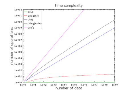
- (4) Example: An algorithm needs to process 1 000 000 elements
- An O(1) algorithm will cost you 1 operation (ex. hash table)
- An O(log(n)) algorithm will cost you 14 operations (ex. well-balanced tree)
- An O(n) algorithm will cost you 1 000 000 operations (ex. an array)
- An O(n*log(n)) algorithm will cost you 14 000 000 operations (ex. best sorting algorithms)
- An O(n2) algorithm will cost you 1 000 000 000 000 operations (ex. bad sorting algorithm)
- (5) Different types of time complexity
- the average case scenario
- the best case scenario
- and the worst case scenario
The time complexity is often the worst case scenario.
- (6) Complexity also works for
- the memory consumption of an algorithm
- the disk I/O consumption of an algorithm
- (7) worse complexities than n^2
- n^{4}: that sucks
- 3^{n}: it’s really used in many databases
- factorial n: never get the results
- n^{n}: ask yourself if IT is really your field
2 Merge Sort
- (1) There are several good sorting algorithms:
- TBD
- (2) Focus on the most important one: the merge sort
- it help use understand a common database join operation called the merge join
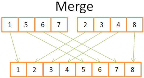
- (3) Merge
- [Costs N operations]merging 2 sorted arrays of size N/2 into a N-element sorted array
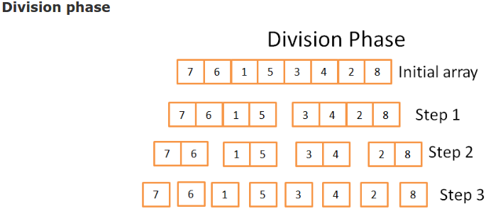
- [Core idea] division phase & sorting phase (divide and conquer algorithms)
- [Steps]
- 1) compare both current elements in the 2 arrays
- 2) take the lowest one
- 3) go to the next element in the array and took the lowest element
- repeat 1,2,3; “never go back”
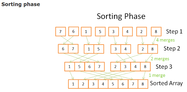
- [overall costs] N * log(N)
- division phase: log(N) steps
- sorting phase: N options of each step
			=======================pseudocode of the merge sort=====================
			array mergeSort(array a)
			   if(length(a)==1)
			      return a[0];
			   end if

			   //recursive calls
			   [left_array right_array] := split_into_2_equally_sized_arrays(a);
			   array new_left_array := mergeSort(left_array);
			   array new_right_array := mergeSort(right_array);

			   //merging the 2 small ordered arrays into a big one
			   array result := merge(new_left_array,new_right_array);
			   return result;
- (4) Why this algorithm is so powerful? Because:
- [in-place algorithm] reduce the memory footprint by directly modifying the input array.
- [external sorting] sorting a multi-gigabyte table, to use disk space and a small amount of memory at the same time without a huge disk I/O penalty.
- [parallel] You can modify it to run on multiple processes/threads/servers. e.g. the distributed merge sort is one of the key components of Hadoop
- [gold] This algorithm can turn lead into gold
3 Array, Tree and Hash table:
The 3 data structures are the backbone of modern databases
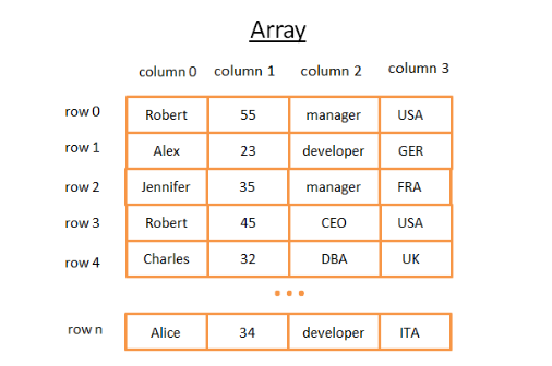
- (1) Array: simplest data structure
- A table can be seen as an array
- [rows and columns]
- Each row represents a subject
- The columns the features that describe the subjects.
- Each column stores a certain type of data (integer, string, date …).
- [Cost] terrible, look for a specific value it sucks (cost N operations)
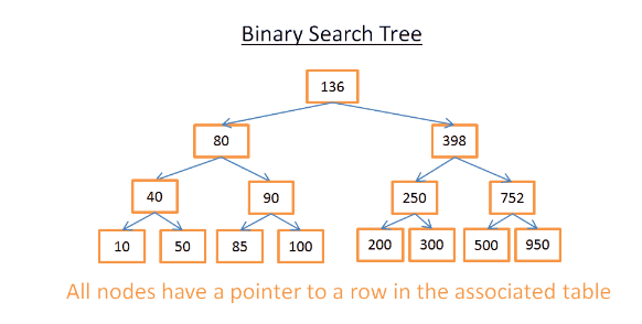
- (2) Tree and database index
- 1) Basics
- [The Idea] the key in each node must be:
- [1] greater than all keys stored in the left sub-tree
- [2] smaller than all keys stored in the right sub-tree
- [Cost] cost of the search is log(N)
- [The Idea] the key in each node must be:
- 2) Database Index
- [Problem] Instead of a stupid integer, you may want to filter records by “Country” with log(N) operations
- [Solution] database index.
- compare the keys (i.e. the group of columns)
- establish an order among the keys
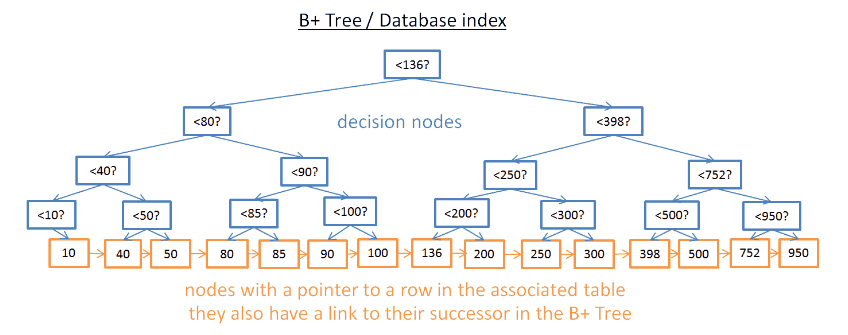
- 3) B+Tree Index O(log(N))
- [Purpose] Range query: instead of getting a specific value, we may want multiple elements between two values
- [Feature] O(log(N))
- [1] only the lowest nodes (the leaves) store information (rows pointers/location)
- [2] the other nodes are just here to route to the right node during the search.
- [3] the lowest nodes are linked to their successors
- [4] more nodes (twice more): decision nodes - help you to find the right node
- [Example] find M successors and the tree has N nodes.
- [Cost] This search only costs M + log(N) operations
- [e.g.] If M is low (like 200 rows) and N large (1 000 000 rows) it makes a BIG difference.
- [Question] If you add or remove a row in a database, what should we do.
- [1] you have to keep the order between nodes inside the B+Tree otherwise you won’t be able to find nodes inside the mess.
- [2] you have to keep the lowest possible number of levels in the B+Tree otherwise the time complexity in O(log(N)) will become O(N).
- [Answer] B+Tree should be self-ordered and self-balanced O(log(N))
- [Consequence] using too many indexes is not a good idea. you’re slowing down the fast insertion/update/deletion of a row.
- [More Details]
- 1) Basics
Note: Considering low-level optimizations, the B+Tree needs to be fully balanced.
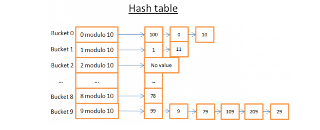
- (3) Hash table
- [Purpose]
- [1] quickly look for values
- [2] it may help us understand a common database join operation, the hash join
- [3] to store some internal stuff (like the lock table or the buffer pool)
- [Idea] The hash table is a data structure that quickly finds an element with its key. To build it
- [1] a key for elements
- [2] a hash function for the keys.
- [3] a function to compare the keys
- [keywords] modulo, bucket
- [Challenge] to find a good hash function that will create buckets that contain a very small amount of elements.
- With a good hash function, the search in a hash table is in O(1).
- [Difference] Array vs hash table
- [Hash Table] A hash table can be half loaded in memory and the other buckets can stay on disk.
- [Hash Table] With a hash table you can choose the key you want
- [Array Table] If you’re loading a large table it’s very difficult to have enough contiguous space.
- [More Details] Java HashMap
- [Purpose]
Global Overview of Database Structure
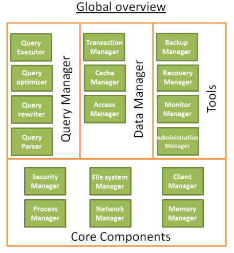
- Multiple components
- A database is divided into multiple components that interact with each other
| Name | Components | Description |
|---|---|---|
| The core components | The process manager | Many databases have a pool of processes/threads that needs to be managed. Moreover, in order to gain nanoseconds, some modern databases use their own threads instead of the Operating System threads. |
| The network manager | Network I/O is a big issue, especially for distributed databases. That’s why some databases have their own manager. | |
| File system manager | **Disk I/O is the first bottleneck of a database. ** | |
| The memory manager | To avoid the disk I/O penalty a large quantity of ram is required. | |
| Security Manager | managing the authentication and the authorizations of the users | |
| Client manager | managing the client connections | |
| The tools | Backup manager | for saving and restoring a database. |
| Recovery manager | for restarting the database in a coherent state after a crash | |
| Monitor manager | for logging the activity of the database and providing tools to monitor a database | |
| Administration manager | for storing metadata (like the names and the structures of the tables) and providing tools to manage databases, schemas, tablespaces, … | |
| The query Manager | Query parser | to check if a query is valid |
| Query rewriter | to pre-optimize a query | |
| Query optimizer | to optimize a query | |
| Query executor | to compile and execute a query | |
| The data manager | Transaction manager | to handle transactions |
| Cache manager | to put data in memory before using them and put data in memory before writing them on disk | |
| Data access manager | to access data on disk |
- (1) Client manager
- [Purpose] it handles the communications with the client.
- [Client Types] a (web) server OR an end-user/end-application
- [API] client managers provide access the database through a set of well-known APIs, JDBC, ODBC, OLE-DB, …
- [Connection steps]
- [1] [authentication] password & rights
- [2] [check] if there is a process (or a thread) available to manage your query.
- [3] [check] if the database if not under heavy load
- [4] [wait] to get the required resources. timeout -> close connection -> errors
- [5] [send] sent you query to the query manager
- [6] [store] query manager stores the partial results in a buffer and start sending
- [7] [stop] stops the connection, give explanation, & releases the resources.
- [Purpose] it handles the communications with the client.
- (2) Query Manager
- [Intro]
- [Important] This part is where the power of a database lies.
- [Functions]
- [Transformed] an ill-written query is transformed into a fast executable code.
- [Executed & Returned] The code is then executed and the results are returned to the client manager
- [Functions]
- [Processes] parsed(valid), rewritten(add/remove), optimized(performance), compiled & executed.
- 1) Query parser
- [Aim] to get an internal representation (tree) of a query
- [Steps]
- [Spelling Errors] wrote “SLECT …” instead of “SELECT …”, the story ends here
- [Keywords Order] keywords are used in the right order.
- [Metadata check] (1)If, the tables exist, (2)the fields of the tables exist, (3)the operations for the types of the fields are possible
- [Check Rights] authorizations to read (or write) the tables (can be set by DBA)
- [Transformed] the SQL query is transformed into an internal representation (often a tree)
- [Sent] the internal representation is sent to the query rewriter.
- 2) Query rewriter
- [Aims] pre-optimize the query, avoid unnecessary operations, to find the best possible solution(help optimizer)
- [Idea] The rewriter applies a list of known (optional) rules to the query.
- [Rules]
- (1) View merging: the view is transformed with the SQL code of the view.
- (2) Subquery flattening: Having subqueries is very difficult to optimize, so the writer will remove the subquery.
- (3) Removal of unnecessary operators: remove DISTINCT, when using DISTINCT & UNIQUE together.
- (4) Redundant join elimination: having twice the same join condition, remove one of them
- (5) Constant arithmetic evaluation: computed once during the rewriting, e.g. WHERE AGE > 10+2 is transformed into WHERE AGE > 12
- (6) (Advanced) Partition Pruning: If using a partitioned table, the rewriter is able to find what partitions to use.
- (7) (Advanced) Materialized view rewrite: modifies the query to use the materialized view instead of the raw tables.
- (8) (Advanced) Custom rules:analytical/windowing functions, star joins, rollup … are also transformed
- [Important] This part is where the power of a database lies.
- prerequisite 3) Statistics
- [Aim] The statistics will help the optimizer to estimate the disk I/O, CPU and memory usages of the query.
- [Basic Statistics] It computes values like
- [1] The number of rows/pages in a table
- [2] For each column in a table:
- distinct data values
- the length of data values (min, max, average)
- data range information (min, max, average)
- [3] Information on the indexes of the table.
- [Example] a table PERSON needs to be joined on 2 columns:LAST_NAME & FIRST_NAME
- the LAST_NAME are unlikely to be the same so most of the time a comparison on the 2 (or 3) first characters of the LAST_NAME is enough.
- join the data on LAST_NAME, FIRST_NAME instead of FIRST_NAME,LAST_NAME
- [Advanced Statistics] histograms: like, the most frequent values, the quantiles, …
- [Aim] to find an even better query plan.specially for equality predicate (ex: WHERE AGE = 18 ) or range predicates (ex: WHERE AGE > 10 and AGE <40 )
- [Where] where can we find the statistics (metadata)
- [Oracle] USER/ALL/DBA_TABLES and USER/ALL/DBA_TAB_COLUMNS
- [DB2] SYSCAT.TABLES and SYSCAT.COLUMNS
- [Must] up to date
- [Disadvantage] takes time to compute. (not automatically computed by default)
- [Improvement] compute the statistics on only 10%. a huge gain in time.
- [However] 10% means a query could take occasionally 8 hours instead of 30 seconds
- [Example] a bad decision: the 10% chosen by Oracle 10G for a specific column of a specific table were very different from the overall 100%
- 3) Query Optimizer:
- [Overview] All modern databases are using a Cost Based Optimization (or CBO) to optimize queries.
- [Three Costs] CPU, disk I/O and memory
- [Note] Each high level code operation has a specific number of low level CPU operations.
- [Three Costs] CPU, disk I/O and memory
- [Indexes] (1) B+Trees(ordered) (2) bitmap indexes, (3) temporary indexes (for the current query)
- [Access Path] Before Join operation, we first need to get data. Ways:
- Full Scan: reading a table or an index entirely
- [Most] the most expensive
- [More] table full scan is more expensive than an index full scan
- Range Scan: need have an index on the field, use a predicate “WHERE AGE > 20 AND AGE <40”.
- [cost] log(N) +M
- [Statistics] Both N and M values are known thanks to the statistics
- [Less] Less expensive in terms of disk I/O
- Unique Scan
- [Situation] need one value from an index
- Access by row id
- [Example] have an index for person on column age
- [valid] SELECT LASTNAME, FIRSTNAME from PERSON WHERE AGE = 28
- [invalid] SELECT TYPE_PERSON.CATEGORY from PERSON ,TYPE_PERSON WHERE PERSON.AGE = TYPE_PERSON.AGE
- ou’re not asking information on person table.
- [Example] have an index for person on column age
- Others paths
- Full Scan: reading a table or an index entirely
- [Join operators]
- [Overview] All modern databases are using a Cost Based Optimization (or CBO) to optimize queries.
- [Intro]